“Liquidity Targeting”: Toward More Efficient Liquidity Mining Programs
By Mechanism Capital
Join the Global Coin Research Network now and contribute your thoughts!
If you’d like to learn about crypto, join our Discord channel and be kept up to date with the latest investment research, breaking news and content, Crypto community happenings around the world!
Introduction
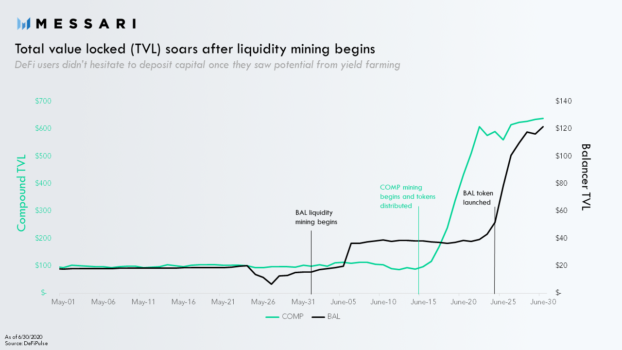
Of the many new trends to emerge in crypto over the past year, Liquidity Mining is doubtless among the most consequential. In 2019, Synthetix became the first large-scale crypto protocol to successfully launch a Liquidity Mining program. But Compound’s June 2020 release of COMP and its accompanying Liquidity Mining program was the true catalyst. In the subsequent months, countless other crypto protocols—from titans like Uniswap and Balancer to microcaps and forks—have utilized some variant of Liquidity Mining. More than just a network-bootstrapping mechanism, Liquidity Mining has quickly become an integral part of token distribution strategies.
The basic insight behind Liquidity Mining is simple: nascent protocols can hit the ground running, as it were, by offering monetary incentives to participants that provide liquidity to the platform, usually in the form of governance/pseudo-equity tokens. As many have noted, Liquidity Mining is just one crypto variant of an incentive strategy frequently employed by companies—think Uber Eats, Seamless, and Grubhub all vying for market share through often-generous promotions.
In this article, we propose a rudimentary quantitative framework for analyzing the necessity and effectiveness of Liquidity Mining programs. This approach—we call it “Liquidity Targeting”—finds an optimal liquidity level for a given protocol and, from there, backs out a Liquidity Mining rewards schedule. For reasons we will discuss, Liquidity Targeting is far from an exact science and should not be treated as such. Nevertheless, we hope that this framework might serve as a quantitative anchor for protocol developers, investors, and community members alike.
Method
The remainder of this article is dedicated to exploring this framework. We begin at the general level, with a discussion of our method, before moving to the more concrete realm with a detailed case study.
Liquidity Targeting has the following steps:
1. For a given protocol’s product offering (e.g. lending/borrowing, stablecoin swaps), determine the market-leading rate of performance (interest rates, price spreads).
2. Establish the liquidity level (i.e. TVL) that is necessary to achieve or surpass the desired rate of performance.
3. Determine the rate of yield (APR) that would attract the requisite liquidity level.
4. If Liquidity Mining is already in use, back out the updated emissions rate that would, at current prices and a target APR, sustain the optimal liquidity level. If Liquidity Mining is not in use and/or if the network token is not in circulation, map out various emissions schedules assuming different token prices.
There are a few wrinkles in this process worth noting.
For one, there may be various metrics by which performance can be measured, leading to more than one “optimal” liquidity level. Moreover, even once a performance metric has been settled on, establishing a target for performance is a purely discretionary matter; a protocol may want to match, marginally surpass, or surpass by a considerable amount the performance levels of competitors.
The third step in the process (establishing a baseline APR) is tricky as well. A confluence of perceived risks—smart contract risk, economic attack vectors, simple price depreciation—will dictate equilibrium APR for each individual protocol.
Last of all, and perhaps most obvious, is the fact that changes in protocol monetary policy do not take place in a vacuum and themselves have reflexive effects. When a revised emission schedule is implemented, the market will likely incorporate this new information into token price. (For example, the decision to reduce Liquidity Mining rewards to target a lower TVL might have the second order effect of increasing the token price, such that even with the lowered emissions, liquidity levels remain mostly unchanged.)
In-depth case study: Curve Finance
In light of these nuances, Liquidity Targeting might appear confusing. Applying this generalized approach to a specific protocol should help to provide a clearer picture.m
Of the many Liquidity Mining programs currently in use, Curve’s is one of the largest and most well-known—and also perhaps the most hotly-contested—rendering it an ideal candidate for this analysis.
Background
Curve Finance is far and away the leading Decentralized Exchange (DEX) on Ethereum for stablecoin and Bitcoin swaps. Unlike Uniswap and other Automated Market Maker (AMM) DEXs which use constant product pricing functions (x * y = k), Curve uses a constant sum function (x + y = k), making it uniquely suited for large trades between equally-priced assets.
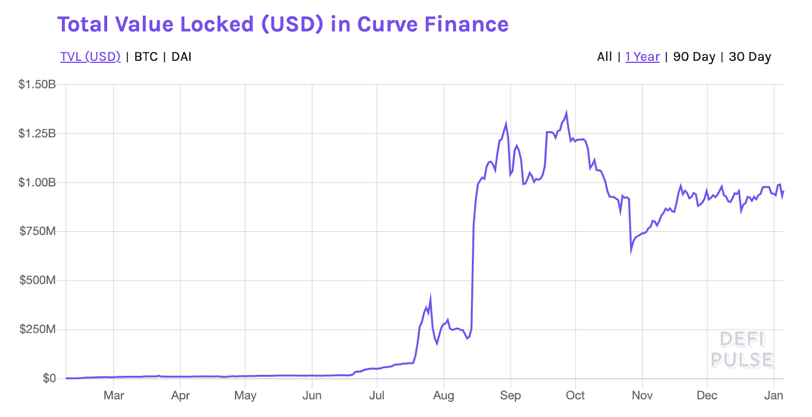
Though Curve’s AMM achieved product market fit without a token, the team decided to launch CRV, the DAO governance token, and an accompanying liquidity mining program in August. Under this program, which is slated to continue for another 350 years, CRV tokens are distributed per day to Curve Liquidity Providers across the various stablecoin and BTC pools.
The launch of CRV generated a frenzy of activity. Eager buyers market bought CRV, pushing the price per token above $50 in the first 24 hours (it now sits around $0.60) and catapulted Curve’s Total Value Locked to over $1.3 billion.
Initially, farming CRV generated three figure annualized yields, but these have since settled to between 5% and 30%, depending on the pool, as CRV prices dropped and Liquidity Providers were diluted via more capital flowing in. Critics and concerned community members alike have noted the continual downward pressure that Liquidity Mining puts on the price of CRV. In response, multiple DAO proposals to materially reduce emissions have been put forward, but none have succeeded.
Because these debates over token distribution and Liquidity Mining programs are often value-laden—and Curve is no exception—we utilized our Liquidity Targeting approach to see if we could provide a more quantitatively-oriented framework. In what follows, we walk through each of the above-mentioned steps as applied to this specific case.
Analysis
Step 1:For the protocol’s product offering, determine the market-leading rate of performance.
As mentioned previously, Curve’s primary product offerings are swaps between stablecoins and BTC on Ethereum. For the purposes of our analysis, we focus on the former.
Before we can settle on a market-leading rate of performance, there is one important preliminary task: determining the trade size Curve should aim to service at an optimal price spread. If Curve’s “product offering” is stablecoin swaps with tight spreads, we need to ascertain which swap size Curve should regularly support before we can calculate the market-leading performance rate (i.e. the lowest trade slippage).
To do so, we tracked stablecoin trades across all of Curve’s pools for a random period of three consecutive days:
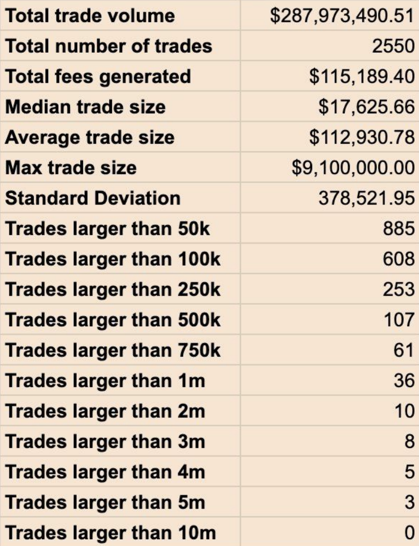
With a sample of just under $300 million in volume and over 2,500 trades broken down by trade size, we can infer that stablecoin trades larger than $1 million are relatively infrequent. Accordingly, we can settle on the $1 million level as the trade size that Curve’s stablecoin pools should aim to service at a market leading rate, as larger trade orders can be split up. It should be noted, of course, that this decision is informed by the data but ultimately discretionary: we could have just as easily settled on $2 million or $500,000 trade sizes.
After landing on a target trade size, we then move to the task of analyzing market performance rates. We compare Curve’s spreads on million dollar stablecoin trades to the performance of other DEXs, CEXs, and a leading OTC desk:
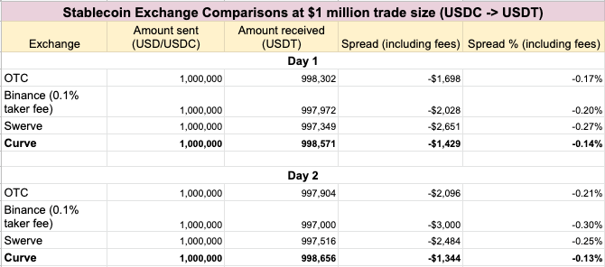
These multi-day snapshots are not comprehensive, but they provide an accurate enough portrait of the stablecoin swap landscape at a $1 million trade size. Curve offers the market leading rate, but not by orders of magnitude. From these data, we can conclude that Curve should target 0.15% spreads (at worst) on million-dollar swaps to retain its edge.
Step 2: Establish the liquidity level (TVL) that is necessary to achieve or surpass the desired rate of performance.
Once we have defined the “desired rate of performance” as maximum 0.15% price spreads on stablecoin trades of $1 million, the next step of the process is to determine how much liquidity Curve needs in order to guarantee this spread, as spreads are ultimately a function of liquidity levels.
At this point in the analysis, we need to get even more granular: each pool on Curve has a different “amplification coefficient” (A), which determines roughly how linear the pool’s pricing curve is. The shape of the curve, in turn, dictates price spreads for various liquidity levels. Among Curve’s stablecoin pools, the yPool, for example, can perform roughly 5x the trade of the 3pool at the same slippage and liquidity level, since the yPool has a higher amplification coefficient.
Because of this additional differentiatingfactor, we cannot simply find a target liquidity level for all stablecoin pools at once, since each will offer different price spreads. Therefore, we focus our analysis on the pool that sees the most throughput of million dollar trades, which happens to be the yPool.
At this point, we have our work cut out for us: we need to establish the TVL necessary for the yPool to sustain 0.15% spreads on $1 million trades.
This stage of the process—working backward from an “optimal rate of performance” to a target liquidity level—is perhaps the most involved. Here, we sought out the assistance of Curve’s founder and CEO, Michael Egorov, who provided us with an elegant, neatly-derived formula for finding an optimal liquidity level based on a target price spread:
L = (S / P) * [6 / (1 + A)]
Where L = the liquidity level for one token in the pool, S= the trade size, P= the desired price spread, and A = amplification coefficient of the pool.
Running the numbers through this formula with the pre-assigned 15 basis point price spread yields a minimum yPool TVL of $16 million. If we were to tighten our spread target even further to 10 bps, the minimum TVL would be $25 million.
It is important to note that the formula assumes a perfectly-balanced pool—which is often not the case in real time. This, in addition to the fact that not all large stablecoin trades are routed through the yPool, explains the seemingly contradictory result that a lower yPool TVL would have tighter price spreads than at current liquidity levels.
Still, the formula enables us to conclude with enough confidence that yPool liquidity—which has been floating in the $100-200 million range for the past few months—is multiples (perhaps even 5-6x) of what it needs to be in order to support million dollar stablecoin trades at the market leading rate.
Step 3: Determine the rate of yield (APR) that would attract the requisite liquidity level.
The penultimate step in the process is to settle on a target yield (APR) that would, all else equal, attract the requisite liquidity. As mentioned above, this particular task is thorny, since Liquidity Mining yield is a function of not only liquidity level and emissions rate, but also token price—which itself is affected by changes to monetary policy.
In theory, one could attempt to derive some sort of broader risk-adjusted rate for crypto yield as a benchmark for yield targeting. Doing so, however, would not be extremely helpful, as each crypto protocol has a unique risk profile that the market alone reflects.
To keep things simple, we chose to settle on a target range that is slightly higher than the current yields in Curve stablecoin pools: 10-15% APR. In practice, this would imply, for example, $20 million in liquidity in the yPool earning 10-15% APR, instead of $150 million in liquidity earning 5-10% APR.
Step 4: If Liquidity Mining is already in use, back out the updated emissions rate that would, at current prices and a target APR, sustain the optimal liquidity level. If Liquidity Mining is not in use and/or if the network token is not in circulation, map out various emissions schedules assuming different token prices.
By this point, we have finished the heavy lifting. All that is left is to calculate the number of tokens distributed weekly to yPool Liquidity Providers. The below matrix shows weekly CRV emissions for various yield and liquidity levels (keeping price constant), with the red box representing our target yield and liquidity level range.
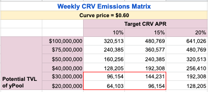
How do we get from the above data—which is specific to the yPool—to a Liquidity Mining rewards schedule for the entire protocol?
Well, a truly comprehensive, protocol-wide Liquidity Targeting analysis would repeat this entire process for each separate pool. However, sparing ourselves this redundant grunt work, we can at least use the yPool data as a rough proxy for Curve rewards as a whole.
Currently, there are just over 5 million CRV distributed weekly to liquidity providers. CRV emissions to the yPool represent only 4% of total CRV emissions (or 200,000 CRV per week), based on the “gauge weights” voted on by governance. From the yPool data alone, we can infer that yPool weekly emissions can be reduced anywhere from 25% to 75%. And if we use the yPool as an approximation, we can tentatively conclude that total weekly CRV rewards can be reduced by a proportional amount.
Concluding thoughts
The bottom line is that Liquidity Mining design matters. Inflationary rewards can be potent weapons for attracting often-fickle liquidity, but they can also prove wasteful when exorbitant or unnecessary. Indeed, there is such a thing as over-incentivization, and the price of this mistake is paid not only by token holders, but also by the protocol itself, since tokens that are misappropriated for existing Liquidity Mining programs cannot be conserved for more useful future incentivization and protocol development purposes. Too often, the marginal cost of Liquidity Mining rewards outweighs the marginal benefit. And of course, the opposite can be true as well: protocols that have failed to bootstrap liquidity through more organic measures would benefit from ramping up incentives.
Attracting liquidity is difficult, and determining how much liquidity is needed is even harder. The process we have outlined in this article is quite involved, even as the methods employed lack scientific precision. Nevertheless, we hope that it can serve as a quantitative foundation for the design and evaluation of both existing and future Liquidity Mining initiatives.
This article was initially published in FTX Monthly Digest‘s December 2020 issue and is re-printed here with the permission of the FTX Digest editors.
-
1244695397@qq.com says:
Suggestions are useful
Leave a Reply
Latest News


More from GCR

Reputation Cookies
This piece was originally published on Decentralised.co. We at GCR will bring to you long forms from Decentralised twice every Month – every alternate Thursday! Decentralised.co ...

GCR Community Events Recap – ...
GCR IRL: GCR at ETHDenver 2024 – The panel discussion at ETH Global Pragma Denver, featuring luminaries like Doug Petkanics from Livepeer, alongside founders from ...

NFT Futures: A New DeFi ...
Summary: Futures, Futures, Futures For a long time in early crypto history, trading was only driven by spot trading where users exchange fiat, other crypto ...